import numpy as np
from scipy.stats import norm

outcomes = [1, 2, 3, 4, 5, 6]
sd = np.std(outcomes)
sd = (1/6)*(1-1/6)
print(f"standard deviation = {sd}")

n_list = [10, 100, 1000, 1000000, 1000000000]

z_99 = norm.ppf(1 - 0.005)  # 99% confidence interval for normal distribution

for n in n_list:
    sd_n = sd / np.sqrt(n)
    conf_range = z_99 * sd_n
print(f"{n:<14} {sd_n:<18.6f} +/-{conf_range:.6f}")2 Rolling Dice
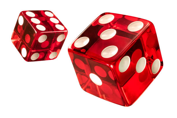
Originally, I thought I’d start this book with a chapter on flipping a coin. That seemed to be the simplest kind of problem to address, but as you’ll see in the next chapter it can become much more complicating than most people suspect. So instead, let’s start with something fairly simple: rolling dice.
2.1 Basics
A single, six-sided die has numbers from 1 to 6 on it. The numbers on opposite sides of the die all add to 7. (1 and 6, 2 and 5, 3 and 4). If we roll this die, we’d expect each side to have an equal probability or landing face up:
\[ P(X=x) = \frac{1}{6} \approx .166667 \quad \text{for } x \in \{1, 2, 3, 4, 5, 6\} \]
In the notation above, \(X\) (upper case) is the random variable being observed and \(x\) (lower case) is the specific outcome: 1, 2, 3, 4, 5, or 6. \(Pr(X=x)\) is the probability that the outcome of the random variable \(X\) is \(x\).
This means that if we rolled the die hundreds, thousands, or millions of times, we’d expect each number to come up 16.67% of the time. This is known as the “law of large numbers.” While there is a high variability for a single roll of the die, we can confidently calculate the average outcome over many trials. Our estimates will become increasingly precise as the number of trials measured increases.
2.2 Averages and the Law of Large Numbers
Actually, the law of large numbers can be applied to this problem in a couple of ways. Oftentimes, it is used to estimate the average of a given value. In this case, if we were to average the numbers that we roll on the die, we would get:
\[ \bar{x}=\frac{1+2+3+4+5+6}{6} = 3.5 \]
The standard deviation for the set of numbers is:
\[ \sigma_{\bar{x}} \approx 1.7078 \]
Over a large number of trials, \(n\), the standard deviation of our estimate of the mean will be:
\[ \sigma_{\bar{x}}(n) \approx \frac{\sigma_{\bar{x}}}{\sqrt{n}} \]
The distribution of the mean, regardless of the underlying distribution or numbers originally, will always tend towards a normal distribution. This allows us to calculate the variability around our estimates of the mean and estimate confidence intervals for different numbers of trials. The code below calculates some of these values and displays them in the table below:
| n | \(\sigma_{\bar{x}}\) | 99% confidence range |
|---|---|---|
| 10 | 0.540062 | +/- 1.391107 |
| 100 | 0.170783 | +/- 0.439907 |
| 1,000 | 0.054006 | +/- 0.139111 |
| 1,000,000 | 0.001708 | +/- 0.004399 |
| 1,000,000,000 | 0.000054 | +/- 0.000139 |
In a similar manner, we can estimate the percentage of times that we expect a given outcome to occur and put confidence intervals around that. To do this, we treat the problem as a Bernoulli process where the only outcome is either 1 (the event is observed) or 0 (the event is not observed). The average value of this outcome over many trials is then the percentage of times that the outcome occurs. This is also our definition of the probability of the event occuring.
The Bernoulli distribution is used to model this type of process. It has a mean of \(p\) and a variance of \(p(1-p)\) where \(p\) is the probability that the event occurs. We can make use of the law of large numbers to calculate standard deviations and confidence intervals for the mean that we would observe (the average number of 1’s in our trials) in exactly the same manner as before, but this time \(\sigma_{\bar{x}}\) represents an average of 1’s and 0’s indicating how many times the specific event occurs. The equation is the same and generates the following results:
| n | \(\sigma_{\bar{x}}\) | 99% confidence range |
|---|---|---|
| 10 | 0.043921 | +/-0.113132 |
| 100 | 0.013889 | +/-0.035775 |
| 1,000 | 0.004392 | +/-0.011313 |
| 1,000,000 | 0.000139 | +/-0.000358 |
| 1,000,000,000 | 0.000004 | +/-0.000011 |
Once again, the variability in our average measured outcome (in this case the percentage of time that we expect a given number to appear on the die) becomes less and less as we increase the number of trials.
2.3 Rolling Two Dice
In many games, players roll two dice and add the sum together. This is a little more interesting. With 6 possible outcomes for the first die and 6 for the second, there are \(6*6=36\) total outcomes. If we are just adding the numbers together then the order of the die doesn’t matter (\(1+6=6+1\)). There are also many different ways to roll some numbers while others only have 1. 2 and 12 for example, only have one combination of values out of the 36 possibilities that produce this sum. The number 7 can be rolled in a variety of ways: 1+6, 2+5, 3+4, and twice this many if we let the order be reversed (6+1, 5+2, 4+3). The probality for rolling each of the possible sums is then:
| Outcome | Ways to Roll It | Probability |
|---|---|---|
| 2 | 1 | \(\frac{1}{36} \approx 2.78\%\) |
| 3 | 2 | \(\frac{2}{36} \approx 5.56\%\) |
| 4 | 3 | \(\frac{3}{36} \approx 8.33\%\) |
| 5 | 4 | \(\frac{4}{36} \approx 11.11\%\) |
| 6 | 5 | \(\frac{5}{36} \approx 13.89\%\) |
| 7 | 6 | \(\frac{6}{36} \approx 16.67\%\) |
| 8 | 5 | \(\frac{5}{36} \approx 13.89\%\) |
| 9 | 4 | \(\frac{4}{36} \approx 11.11\%\) |
| 10 | 3 | \(\frac{3}{36} \approx 8.33\%\) |
| 11 | 2 | \(\frac{2}{36} \approx 5.56\%\) |
| 12 | 1 | \(\frac{1}{36} \approx 2.78\%\) |
Notice that 7 is the most likely outcome when you roll two dice.
We’ll have more fun with this later when we look at Craps, but this is probably enough for now. Let’s move on to something that seems simple, but can actually be quite interesting: flipping a coin.